

Palaeoclimate and fossil woods—is the use of mean sensitivity sensible?
MARC PHILIPPE
Philippe, M. 2023. Palaeoclimate and fossil woods—is the use of mean sensitivity sensible? Acta Palaeontologica Polonica 68 (4): 561–569.
The growth rings of fossil wood provide valuable data on tree ecology. As many of the parameters controlling width are climatic, it is tempting to use these rings as an indicator of climate. This is what has been done, with great success, by dendrochronological studies of archaeological wood. For wood dating from before the Pleistocene, however, the task is more uncertain. Since around 1980, researchers have relied mainly on a statistical parameter, the mean sensitivity, an average of the difference in width between two consecutive rings. However, there has never been a critical examination of utility and significance of this parameter for fossil wood. I compiled 63 studies that used mean sensitivity for palaeoclimatological inferences. An analysis of this compilation is presented here. Despite its ups and downs since the 1980’s, mean sensitivity is increasingly used by palaeobotanists. However, it has been used in very different ways. The values obtained for the same fossil can vary greatly from one researcher to another, but also according to the radii of the woody axis considered. Within fossil wood assemblages, average sensitivity varies widely, but rarely consistently. Overall, mean sensitivity values are continuously, normally and unimodally distributed, and therefore are unsuitable for characterising discrete climate classes. Finally, it seems that the most recent studies are also the least cautious when it comes to interpreting the values obtained.
Key words: Climate proxy, growth ring, palaeobotany, palaeoecology, tree.
Marc Philippe [marc.philippe@univ-lyon1.fr; ORCID: https://orcid.org/0000-0002-4658-617X ], Univ Lyon, Université Claude Bernard Lyon 1, CNRS, ENTPE, UMR 5023 LEHNA, F-69622, Villeurbanne, France.
Received 27 September 2023, accepted 14 November 2023, available online 19 December 2023.
Copyright © 2023 M. Philippe. This is an open-access article distributed under the terms of the Creative Commons Attribution License (for details please see http://creativecommons.org/licenses/by/4.0/), which permits unrestricted use, distribution, and reproduction in any medium, provided the original author and source are credited.
Introduction
Almost all trees produce wood rhythmically, and the amount they produce during a growing season depends pro parte on climatic parameters, such as rainfall and temperature (e.g., Mundo et al. 2012; Prior et al. 2012; Wunder et al. 2013). Therefore, it is sensible to use the characteristics of this growth as an annual record of the climate. Dendrochronology uses growth ring width sequences to date and correlate archaeological woods, geological events or to follow the evolution of climates, with remarkable efficiency.
In deeper times, wood is a common fossil from the Devonian period onwards, and from that time it shows growth rings (secondary xylem increments), which can be interpreted as characterising a rhythmic growth. It is thus tempting to interpret the characteristics of these rings in terms of palaeoclimatology. Both qualitative and quantitative approaches have been proposed for fossil woods (Creber and Chaloner 1987), i.e., woods dating from the Pleistocene or older. The mean-sensitivity (MS) is probably the most used quantitative approach.
The mean sensitivity, or mean annual sensitivity, is a parameter originally designed by Andrew E. Douglass to discard tree ring sequences not suitable for a dendrochronological approach (Douglas 1928, 1936). The MS is an average of the relative differences in thickness of a series of pairs of consecutive growth rings. Below and above arbitrarily chosen thresholds, MS characterises growth ring width series where the climatic signal is too uniform or too distorted by other ecological factors to be used for dendrochronological correlations. The use of MS for dendrochronology was greatly popularised in 1976 by a textbook authored by Harold C. Fritts (see also Fritts and Shatz 1975).
Shortly after this date, Geoffrey Creber proposed to extend the use of this parameter to fossil wood dendroclimatology (Creber 1977). For him the complacency of rings sequences invalidates a dendrochronological approach but would demonstrate the constancy of climate (Creber 1977). However, Creber himself did not use the MS in his own works on dendroclimatology (e.g., Creber and Chaloner 1984, 1987). The MS was first used for palaeoclimatic deductions from Mesozoic fossil woods by Jefferson (1982). Since then, MS of fossil woods of different ages has been used regularly as a palaeoclimatological proxy (e.g., Francis 1984, 1986; Falcon-Lang and Cantrill 2002). There has been a rapid shift from Creber’s cautious use of MS to publications claiming, for example, that a high MS characterises variable climates (Parrish and Spicer 1988; Spicer and Parrish 1990; Da Rosa Alves and Guerra-Sommer 2004).
Dozens of papers have used MS to interpret fossil wood growth rings in terms of palaeoclimate since 1982. The repeatability and validity of this approach, both at the sample and assemblage level, were questioned (Poole and Bergen 2006 and references therein). However, there has been no comprehensive review of this body of works using the MS or a critical evaluation of the utility of this parameter for palaeoclimatic studies. Here I review the use of MS for palaeoclimatological inferences from fossil wood and question its significance and efficacy.
Abbreviations.—AS, annual sensitivity (Fritts 1976); CV, coefficient of variation, the ratio of the standard deviation to the mean; MAR, mean annual rainfall (mm); MAT, mean annual temperature (°C); MS, mean sensitivity (Fritts 1976); RD, relative difference; SM, simple arithmetic mean; WM, weighted arithmetic mean.
Material and methods
On the 5.07.2023 Google Scholar was searched with the key words “fossil”, “wood” and “mean sensitivity”. All the academic sources giving values of MS for Pliocene or older woods were compiled. Sources from my own bibliography, where Mesozoic woods are over-represented, were added. All together 63 studies were taken into account. The table sums up this database (see SOM, Supplementary Online Material available at http://app.pan.pl/SOM/app68-Philippe_SOM.pdf).
The database was analysed from different perspectives. The temporal distribution of the studies was first examined, looking for possible influences of one (or more) particular study on the others. The different ways that were used to calculate MS were then considered. It was revealed that the MS of the same fossil wood specimens were calculated independently by three researchers (Jefferson 1982; Chapman 1994; Falcon-Lang et al. 2001), offering the opportunity to test inter-individual MS measuring repeatability. Repeatability was also addressed by some studies that evaluated MS variations when calculated on different radii of the same fossil (Jefferson 1982; Brea et al. 2008), or on different parts of the same species (Fletcher et al. 2015). The MS value variability for the different fossil wood specimens of an assemblage were then analysed, notably using the coefficient of variation (CV), i.e., the ratio of the standard deviation to the mean, expressed as a percentage.
Results
The temporal applications of the mean sensitivity.—The number of publications using the MS for palaeoclimatological inferences has clearly fluctuated (Fig. 1), with an overall increasing trend. Even if the pattern is corrected for this trend, which is probably linked to the overall inflation of the annual number of scientific publications, the curve peaks and declines.
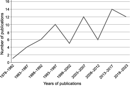
Fig. 1. Number of publications using MS from fossil woods for palaeoclimatological inferences in the database (see SOM).
It was the pioneering work of Geoffrey Creber (1977) that initiated the application of MS to the study of fossil woods. This work inspired Jefferson (1982) and later (Francis 1984, 1986) and soon other researchers. However, by the end of the twentieth century MS became less commonly used. The works of Falcon-Lang (Falcon-Lang et al. 2001; Falcon-Lang and Cantrill 2002) seems to have momentarily revived interest in MS in the early 21st century. During the 2008–2012 interval, however, the number of publications using MS dropped again, possibly as a consequence of the cautionary results of Falcon-Lang (2005a, b; for details see below). In the last decade, eventually, palaeoclimatological inferences from fossil woods based on MS have become common again. However, my literature review does not identify any triggering factors for this resurgence. Such a contrasting pattern suggests that the use of MS for palaeoclimatic inferences has not established itself as an unavoidable and widely accepted method. Some work carefully avoids it (e.g., Poole et al. 2005).
Different ways to calculate mean sensitivity.—As explained by Fritts (1976: 258) “the average mean sensitivity (MS) for a series is calculated as follows:

where Xt is each datum and the vertical lines designate the absolute values of the term enclosed by them”. Fritts (1976: 258) then adds “The values of mean sensitivity range from 0 where there is no difference to 2 where a zero value occurs next to a nonzero one in the time sequence”. The MS could indeed be equal to 0 if all ring widths are exactly the same. It is more difficult to imagine a growth-ring with no width. If all width differences of consecutive ring pairs tend to infinity, then the MS tends to 2; however, this is clearly only a theoretical possibility.
The MS is thus an average, for a series of n rings, of the n-1 absolute values taken by annual sensitivity (AS), i.e., the relative differences in ring width of the n-1 consecutive ring pairs. Modified versions of the MS have been proposed (Schulman 1956; Fürst 1963) but to my knowledge never used for fossil woods.
According to Poole and Bergen (2006: 179–180), when extending the growth ring analysis approach to pre-Quaternary isolated wood material ideally five prerequisites need to be met: (i) assemblages need to be of an adequate sample size (ca. >20 trees) and taxonomically diverse; (ii) specimens should be identifiable in terms of taxon and ontogenetic age; (iii) organs should be of complete cross section and have similar origins (with preference for trunk wood) and excluding the inner xylem near the pith to overcome problems of rapid initial growth, confused growth interruptions and unequal gravitational effects; (iv) taxa should be “reliable”; (v) conifer taxa need to have known leaf longevity/retention times.
Unfortunately, these five prerequisites cannot easily be fulfilled. It is the case in a small percentage only of the references listed in studied database.
Falcon-Lang (2003) and later Davies-Vollum et al. (2011) and Benicio et al. (2016) used MS in an unconventional manner, to measure spacing variability of growth interruptions in woods where true annual rings (i.e., rings continuous around the tree circumference and having a distinctly asymmetric boundary) are not present, or in woods where true and false rings co-occur. In a hand specimen, where the whole tree circumference usually cannot be explored, it is often difficult to decipher between true rings and false rings (growth interruptions). Most publications do not make it clear whether false rings were taken into account in the calculation of MS.
Parrish and Spicer (1988) calculated MS for fossil woods deformed by taphonomical processes with measured ring thickness values and then with restored values, which they derived by using the upper limit of the estimated deformation. Differences between the two calculations were less than 10% in all cases.
Chapman (1994) calculated MS for an Alaskan Cretaceous wood using ring widths measured either in number of cells or in µm. MS values were 10% higher in the second case. Ruiz et al. (2020) specified the threshold, in number of rings present, that they consider necessary to be able to calculate a MS, but few other works do the same, and the MS has sometimes been calculated on series of less than 20 rings.
More recently, Esperança Júnior et al. (2023) have used the MS in a highly unusual way. Arguing that the Permian woods they studied do not have annual rings (although they illustrate convincing growth stoppages in their fig. 3), they calculate the MS not from the width of pairs of successive rings but from pairs of successive cells. They state that they are aware of the time-scale problem this entails, but nevertheless use the MS values calculated for palaeoclimatic deductions.
Interestingly, MS values were reported for the same fossil wood assemblage, from the upper Albian Triton Point Formation of Alexander Island, Antarctica, by Jefferson (1982), Chapman (1994) and subsequently Falcon-Lang et al. (2001). Comparison (Table 1) reveals that the values given for the MS of the same samples may differ by up to 27% between authors, suggesting that observer bias may be significant.
Table 1. Number of observed rings and mean sensitivity (MS) for samples studied by Jefferson (1982) from Triton Point Formation, upper Albian (Lower Cretaceous), Alexander Island, Antarctica, and the value given by Chapman (1994) and Falcong-Lang et al. (2001) for the same samples.
|
Sample code (British Antarctic Survey) |
||||||
|
Number of rings measured |
MS |
Number of rings measured |
MS |
Number of rings measured |
MS |
|
|
KG2821.86 |
not taken into account |
14 |
0.58 |
not taken into account |
||
|
KG2821.97 |
13 |
0.393 |
17 |
0.50 |
16 |
0.499 |
|
KG1702.6 |
43 |
0.621 |
53 |
0.61 |
48 |
0.573 |
|
KG2814.254 |
43 |
0.404 |
48 |
0.41 |
45 |
0.385 |
|
KG2817.20 |
not taken into account |
90 |
0.33 |
not taken into account |
||
This also raises the question of the variability of the values obtained depending on where in the fossil wood specimen the ring thicknesses are measured.
Interestingly, in her approach, Fletcher gave not only MS values, but also standard-deviation for AS (Fletcher et al. 2015). Although standard-deviations were somewhat laborious to compute in the seventies, it is now fairly easy and adds much interest to a single mean value as the MS. Francis (1984) also indicated that MS should not be discussed without previous discussion of AS, noting that even though a tree may have an overall “sensitive” mean sensitivity, it may have a greater number of “complacent” values of annual sensitivity, and vice versa.
Intraspecific mean sensitivity variability.—Chapman (1994) calculated MS for an Alaskan Cretaceous fossil branch for both normal wood and reaction wood. She found little difference (MS 2% higher in the second case). MS is not supposed, however, to be calculated on something other than trunk wood, and especially not on a plagiotropic axis (Fritts 1976). Fletcher et al. (2015) compared the MS of different samples, all belonging to the same species and the same fossil assemblage, but to different tree parts. Their results are not statistically significant (Table 2); however, they suggested that MS calculated from roots are higher than those calculated from stump or trunk pieces.
Table 2. Mean sensitivity (MS) for different tree parts of Protophyllocladoxylon owensii Fletcher, Cantrill, Moss, and Salisbury, 2014, Upper Cretaceous, Australia. Data from Fletcher et al. (2015).
|
Plant part |
Number counted |
Minimum MS |
Average |
Maximum MS |
|
Trunk |
5 |
0.27 |
0.34 |
0.46 |
|
Stump |
4 |
0.16 |
0.38 |
0.76 |
|
Root |
2 |
0.53 |
0.56 |
0.6 |
|
Total |
11 |
0.16 |
0.39 |
0.76 |
Jefferson (1982) calculated MS along different radii for four Cretaceous woods from the Antarctic and Brea et al. (2008) performed a similar calculation on woods from the Triassic of Argentina (Table 3). The relative difference (RD), expressed as percentage, is calculated as:
RD = 200 (M – m)/(M + m)
where M is the highest calculated MS for a fossil wood specimen and m the smallest.
RD does not seem to be correlated to the number of radii considered. It reaches 76% in the cases where two radii were considered and up to 90% in cases when more than two radii were considered. In less than 10% of the cases was RD <10%. As a rule, MS is thus variable according to the radius considered.
Kłusek (2006) revealed that MS is quite sensitive to the irregular occurrence of very high AS coefficients within the ring sequences of analysed fossil wood specimens.
Table 3. Values of mean sensitivity (MS) calculated along different radii of the same sample for woods from the Cretaceous of Antarctica (data from Jefferson 1982) and from the Triassic of Argentina (Brea et al. 2008).
|
Source |
Sample code |
Number of radius considered |
Minimum MS |
Maximum MS |
Relative difference (%) |
|
KG2815.256 |
2 |
0.373 |
0.434 |
15 |
|
|
KG2816.39 |
3 |
0.339 |
0.430 |
24 |
|
|
KG2817.16 |
2 |
0.423 |
0.492 |
15 |
|
|
KG1719.3 |
2 |
0.420 |
0.442 |
5 |
|
|
LPPB12604 |
4 |
0.26 |
0.32 |
21 |
|
|
LPPB12605 |
2 |
0.21 |
0.24 |
13 |
|
|
LPPB12606 |
4 |
0.14 |
0.37 |
90 |
|
|
LPPB12609 |
5 |
0.31 |
0.37 |
18 |
|
|
LPPB12610 |
5 |
0.20 |
0.38 |
62 |
|
|
LPPB12612 |
2 |
0.20 |
0.29 |
37 |
|
|
LPPB12613 |
2 |
0.28 |
0.62 |
76 |
Mean sensitivity at the fossil wood assemblage level.—The relationship between tree rings and climate has long been demonstrated to be variable, at the inter-individual level within a given species, and at the interspecific level (Fritts 1976; Tessier 1989).
When dealing with a fossil wood assemblage, there is always a trade-off to be found between increasing the number of samples to be included in the calculation of the average MS for the assemblage and the risk of including a sample that is quite different from the others for this parameter. This is especially true since fossil wood assemblages are commonly limited in the number of samples suitable for such analyses. Parrish and Spicer (1988) showed that the average MS increased from 0.37 to 0.42 (+14%) by including a seventh sample to their assemblage of six woods, as this last one is atypical. Sporadic seasons of high or low growth rates strongly skew mean sensitivity towards the sensitive field even if most analysed ring-series show a complacent response to interseasonal environmental conditions (Zamuner 1986; Weaver et al. 1997).
Before analysing the MS of a fossil wood assemblage, the first prerequisite of Poole and Bergen (2006: 179–180) should be remembered, i.e., (i) assemblages need to be of an adequate sample size (ca. >20 trees) and taxonomically diverse. Taphonomy should also be studied as, although most significant log accumulations were probably rapidly deposited and concerned trees originating from an ecologically homogeneous area, this might not always be the case (Philippe et al. 2022).
Falcon-Lang et al. (2001) calculated MS for a wood assemblage from the Cretaceous of Antarctica and then calculated a simple arithmetic mean (SM) of the MS values, as well as a weighted mean (WM), weighted in proportion to the number of rings measured in each wood sample. SM and WM differed little for a first wood set with high MS (0.42 vs 0.44; 1330 rings measured, on average 40 rings per sample) but they differed more for a second wood set (0.28 vs 0.33; 318 rings counted on average 20 rings per sample). This suggests that, at least for this case, the more rings are measured per sample, the lower the MS.
Falcon-Lang (2005a,b) demonstrated that there is a significant ontogenetic trend for anatomical parameters, such as tracheid pit distribution, cross-field pit frequency, ray dimensions, ray spacing, tracheid diameter, mean ring width and mean sensitivity. Mean sensitivity increases with decreasing ontogenetic age (r² = 0.556), with lower trunk discs having values around 0.22–0.27 compared with upper trunk values ranging up to 0.43, almost 100% more.
Röβler (2021) calculated MS for different systematic groups within an early Permian fossil wood assemblage from Germany (Table 4). The values differ greatly, despite that these trees grew in the same ecosystem, with MS being equal to 0.35 for gymnosperms, 0.44 for calamitaleans and as much as 0.48 for medullosans ferns.
Table 4. Mean sensitivity (MS) values for different informal taxonomic groups in an fossil wood assemblage from lower Permian Germany. Data from Röβler (2021).
|
Taxon |
Minimum MS |
Mean MS |
Maximum MS |
|
Medullosan seed ferns |
0.31 |
0.48 |
0.77 |
|
Calamitaleans |
0.27 |
0.44 |
0.72 |
|
Pycnoxylic gymnosperms |
0.24 |
0.35 |
0.77 |
|
All taxa |
0.24 |
0.41 |
0.77 |
Table 5. Comparisons of the mean sensitivity (MS) (average and standard deviation) for different subsets of a wood assemblage from the Triton Point Formation, upper Albian, Lower Cretaceous, Alexander Island, Antarctica, in studies by Jefferson (1982), Chapman (1994), and Falcon-Lang et al. (2001).
| |
|||
|
Number of studied samples |
2 |
5 |
49 |
|
Mean MS |
0.418 |
0.486 |
0.372 |
|
Standard deviation |
not calculated |
0.117 |
0.112 |
As described above, MS values were reported for the same fossil wood assemblage by Jefferson (1982), Chapman (1994) and Falcon-Lang et al. (2001). At the assemblage level, the values given by Jefferson on the basis of two samples yielded a mean MS for the assemblage of 0.418, whereas Chapman on the basis of 5 samples calculated a mean MS of 0.486, and Falcon-Lang et al. of 0.372 (Table 5).
With this data set (Table 5) it would be expected that the higher the number of studied samples in a wood assemblage, the lower the calculated MS. However, a synthesis from the bibliographical survey revealed no correlation between MS value and the number of samples considered (Fig. 2).
Luthardt and Röβler (2017) used the MS in the most orthodox way, i.e., to sort the 11 best fitting series out of 43 tree-ring series measured from a fossil wood assemblage dated from the Permian. These eleven series were then used to calculate a mean curve which evidenced a ca. 11 year cyclicity, similar to that induced in modern trees by sunspot activity. It must be emphasized that Luthardt and Röβler (2017) studied an exceptional palaeontological object, a forest fossilized instantaneously in situ by a rapid succession of pyroclastic surges and flows. Most “petrified” forests are, however, assemblages of dead logs of various provenance in fluvial or coastal settings. Only much less precise information can be expected from a MS study of ring variability in such assemblages.
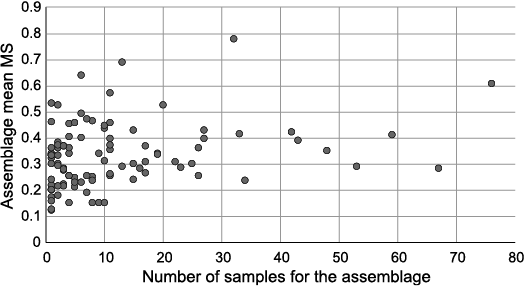
Fig. 2. Mean MS for fossil wood assemblages in studied database as a function of assemblage size, in number of samples measured.
Discussion
When reading the corpus of articles, one is struck by three facts: (i) the repetitiveness of the MS chapter sentences, not commented here; (ii) the fact that few works use the post-1977 results of dendrochronologists; (iii) the uniformity of the vast majority of conclusions. However, one can discern a shift between the cautiousness with which the older works make inferences and the much more peremptory character of some of the more recent ones.
Lessons from the present.—As early as 1989, dendrochronologist Lucien Tessier (1989: 517) came to the conclusion that “The regional climate, the microclimate, the ‘operational environment’ (…) as well as physiological and biological processes governing growth, which are dependent on the genotype of the species, are involved in ring—climate relationship”. Tessier (1989) insisted on the different scales at which climate must be considered. The growth in diameter of a tree and, therefore, the measurable MS in its various woody parts, responds to these different scales. MS based conclusions, such as “these trees grew under changing climate” ignore the scale question and are, therefore, almost meaningless. Moreover, Briffa et al. (1998) warned that temperature sensitivity changed in recent time, as it probably also did in the past, all the more as atmospheric CO2 concentration is by no means a constant through geological times, which might have influenced tree growth (Osborne and Beerling 2002). This suggests that MS threshold values, elaborated in the 1950’s for extant trees, are possibly not relevant for the Mesozoic or older periods.
Falcon-Lang (2005a) studied MS from a database with raw mean ring width data sets of 727 sites distributed worldwide (with a strong bias towards boreal settings). He concluded (Falcon-Lang 2005a: 438) that there is “no evident relationship between MS and any individual climate parameter”. Such a conclusion could be considered as quite predictable as all the climate parameters he considered are mean annual values (such as MAT, Mean Annual Temperature; and MAR, Mean Annual Rainfall) and MS is also an average. However, Falcon-Lang (2005a) also observed that, for conifers in cool-to-cold and dry regions, the MS range is greater (0.15–0.75) than in hot and wet regions (0.17–0.35). Conversely, plotted against the MAT/MAR climate index, angiosperm MS values produced a more or less random scatter. These results raised interrogations which possibly explain the relative drop in the number of publications using MS during 2008–2012 interval.
Later on Lieubeau et al. (2007) revealed that for a set of New Caledonian Araucariaceae, ring width is more strongly impacted by extremes and monthly temperatures and rainfall amounts than by yearly values. This contribution also evidenced that discarding false rings allows better correlation with climate parameters, such as the total rainfall during the growth season. This fully endorses Poole’s (Poole and Bergen 2006: 180) third prerequisite: “(iii) organs should be of complete cross section…”.
According to Francis (1986: 678), for some modern Araucaria araucana trees growing under temperate climate, in Argentina, “values of MS were also very low, ranging from 0.12 to 0.23, illustrating that growth was very uniform from year to year”. Interestingly, Boswijk et al. (2014) compiled data for 201 kauri trees (Agathis australis) from the New Zealand North Island, either living or subfossil. They found that their MS spanned a large range from 0.075 to 0.675, with a mean at 0.315, and an almost normal distribution. Together with the results of Lieubeau et al. (2006), it suggests that modern Araucariaceae of low and mid-latitudes behave quite differently in regard to MS.
Guiot (1987), studying Picea mariana individual series sampled in northern Quebec, revealed that MS increased more than twofold after 1860 because of a climatic improvement, i.e., a releasing of temperature stress. Colangelo et al. (2018) noted in Italy that declining and non-declining oaks (Quercus pubescens and Q. cerris) severely stressed by climate change all have statistically similar MS (ca. 0.33), differing by less than 3%. In Mexico, Correa-Diaz et al. (2018) measured MS at 0.39 +/- 0.04 for a set of Taxodium mucronatum trees submitted to a stress due to contemporaneous rise in atmospheric CO2 concentration and concordant temperature increase.
For modern conifers growing in semi-arid climates Fritts el al. (1965) calculated a mean sensitivity of 0.58 for those trees growing near the forest border, whereas those growing in the forest interior had values around 0.22.
Almost since it was established, mean sensitivity has been criticized. Indeed, mean sensitivity as defined by Fritts (1976) is often proportional to the standard deviation of the ring width, and it is ambiguous, because it does not separate variance and autocorrelation (Jansman 1995; Ricker et al. 2020). This is why a probabilistic version of the mean sensitivity was proposed by these authors. To the best of my knowledge, it has not yet been used for fossil woods.
Some conclusions based on a study of the MS of fossil woods are weakened by ignoring the limitations suggested by the study of extant woods. The results of those studies, which merely repeat the interpretative schemes of Parrish and Spicer (1988), might have to be reconsidered.
Similar conclusions.—The question arises as to whether MS values originally considered to characterise a tree-ring series that does not reliably record climate could paradoxically be used for palaeoclimatic deductions at assemblage level, i.e., when a set of samples for a given locality is considered.
I calculated the mean MS for 99 fossil wood assemblages. The value distribution (Fig. 3) is unimodal and normal (not tested statistically). Observed MS range from 0.123 to 0.778, whereas for modern trees most MS fall within the range 0–0.6 (Creber 1977). Here, almost two-thirds (64%) of fossil wood assemblages that have been studied have a mean MS sandwiched between 0.2 and 0.39, and thus give similar conclusions. This could be due to the homogeneity of the hydrological conditions under which these series of growth rings were generated, with upland floras less likely to be fossilised than others.
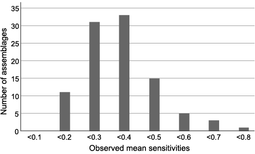
Fig. 3. Distribution of mean MS values for the 98 fossil wood assemblages of studied database (percentages of the total number).
When applying MS approach to fossil woods, all authors have used a threshold proposed by Creber (1977). When MS is less than than 0.3 corresponding growth ring series are described as “complacent” whereas, above this value, the series are described as “sensitive”.
Not all the series measured along different radii of a given log necessarily fall into the same category (Douglas 1928). A first level of integration is then to consider as “complacent” trees which have mostly or exclusively MS <0.3, and “sensitive” trees which have mostly or exclusively MS >0.3. At a second level of evaluation complacent trees are said to have little response to climate, whereas the sensitive ones better record climatic variation (Francis 1984). A third, and obviously strongly hypothetical assessment, is to consider that woods with MS less than 0.3 probably grew in relatively constant and equable environments, whereas those with MS >0.3 had a different origin and “probably grew in variable environments” (Parrish and Spicer 1988; Martinez et al. 2023).
For 43% of the assemblages mean MS is lower than 0.3, i.e., the threshold proposed by Creber (1977). This would mean that 43% of the wood studied, of all ages and origins, would have formed under a constant and equal climate. This may seem like a lot, but it is virtually impossible to test the plausibility of this assertion. It could mainly reflect the homeostatic capacities of forest ecosystems more than a global feature of palaeoclimates. There is nothing in the studies analysed to suggest a less arbitrary threshold.
Overall the MS values are continuously, normally and unimodally distributed, and it is, therefore, difficult to use them to characterise hypothetical discrete climate classes based on interannual climate variability. It doesn’t seem very sensible to think of characterising the climate in a univocal way with MS as the only indicator, itself a summary of the inter-annual (or inter-seasonal) variability of the tree’s growth, given the complexity of tree’s growth-climate relationship.
I calculated the coefficient of variation (CV is defined as the ratio of the standard deviation to the mean expressed as a percentage) from the compilation (Fig. 4). The CV reaches 63% and is greater than 33% in 57% of the cases. Such CV values suggest that most corresponding assemblages are probably too heterogeneous for any assumption. There is no obvious relationship between the mean sensitivity, CV, and the number of samples of the assemblage.
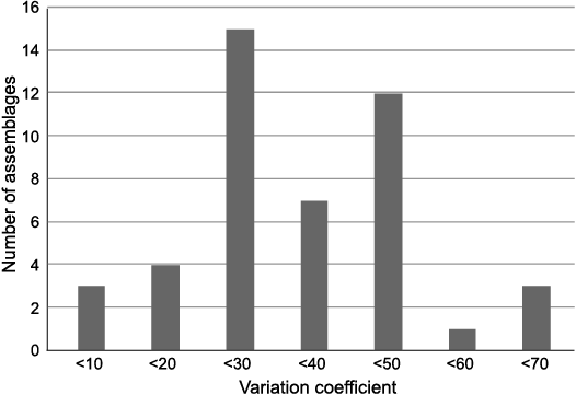
Fig. 4. Distribution of mean CV (ratio of the standard deviation to the mean) for MS values of 61 fossil wood assemblages of studied database.
Shift in formulation.—It may be artificial, but it would be interesting to compare the formulations of three articles regarding the interpretation of the values obtained for the MS. Parrish and Spicer (1988: 24) stated that “Woods with MS less than 0.3 […] probably grew in relatively constant and equable environments, whereas those with MS> 0.3 […] probably grew in variable environments”. Later Tilley indicated (2016: 181; see also Tilley et al. 2014) that “[for a tree, MS] values greater than 0.3 indicate growth under a fluctuating climate (sensitive growth), and values below indicate growth under an equable climate (complacent growth).” For Ruiz et al. (2020), “a [MS] value of 0.3 is taken to distinguish between “complacent” trees that grew under a favourable and uniform climate (MS < 0.3) from those that are “sensitive” to fluctuating climate parameters (MS > 0.3).”
At the assemblage level, climate is regularly interpreted as stressing when the mean MS exceeds 0.3, even if several woods in the assemblage have much lower MS (0.1–0.2) (see e.g., Artabe et al. 2007). Inferences such as “The relatively high mean sensitivity (MS average of 0.4) of fossil woods indicates that trees were influenced by monsoon climate during the growth period, and the environment was very unstable with uneven annual precipitation” (Wei et al. 2016: 1771), or “Mean sensitivity analysis of growth rings in the stumps indicates small-scale environmental disturbances on the floodplain, such as periodic flooding, or regional environmental disturbances, such as volcanism, disrupted wood production.” (Davies-Vollum et al. 2011: 89), might be based on over-interpretation.
Although this is not quantifiable, the impression a palaeoxylologist obtains from reading the articles in my database is that interpretation of MS values has become progressively less cautious.
Conclusions
The statement that “Growth rings in fossil woods provide invaluable data concerning tree ecology” (Falcon-Lang et al. 2004: 45), under this wording or another, is regularly repeated in several MS-based discussions. However, the fact that this statement is fundamentally true does not imply that the data can be interpreted uncritically. Already in 1989, Tessier warned that, however attractive it may be, a quantitative reconstruction of the climate based on tree-ring variability has its limitations. Without putting it into perspective, it constitutes falsely absolute information.
Mean sensitivity is an unsophisticated statistical tool for analysing growth variability. Neither the appearance of science suggested by the way the MS formula is written, nor a fascination with quantification, exonerate us from the need for caution when interpreting MS data from fossil wood. A probabilistic approach might be preferred (Ricker et al. 2020).
There is a short-sightedness in ignoring the fact that the local climate recorded by the rings of a given tree, or a few trees, is not the regional climate and even less the global climate. Eventually, samples preserved in alluvial to marine deposits might derive from a range of ecosystems (McLoughlin 1996) making mean sensitivity analysis sensible at assemblage level only if sedimentology can demonstrate that only one type of vegetation yielded the fossil woods.
This call for caution in the use of MS for the palaeoecological interpretation of fossil woods should not obscure the fact that they can be validly used to for a range of palaeoenvironmental applications, including: estimating ancient forest stature and productivity (e.g., Williams et al. 2009; Pole 1999), tree architecture (Steart et al. 2023), insect, fungal, and bacterial interactions (Feng et al. 2019; McLoughlin and Mays 2022; Greppi et al. 2022), tracking taphonomic pathways (Philippe et al. 2022), growth disturbances from volcanic activity (Cuneo 2021), palaeoseismicity (Minor and Peterson 2016) and insect defoliation (Dechamps 1984), detecting palaeo-rainshadow effects (Oh et al. 2020) and biogeographic patterns (Philippe et al. 2004).
Acknowledgements
Thanks to Tamara Fletcher (University of Leeds, UK) for her clarification on her MS calculation and to the several colleagues who kindly sent their papers. Marion Bamford (Witwatersrand University, Johannesburg, South-Africa) and four anonymous reviewers greatly improved a previous version.
References
Artabe, A.E., Spalletti, L.A., Brea, M., Iglesias, A., Morel, E.M., and Ganuza, D.G. 2007. Structure of a corystosperm fossil forest from the Late Triassic of Argentina. Palaeogeography, Palaeoclimatology, Palaeoecology 243: 451–470. Crossref
Benício, J.R.W., Spiekermann, R., Manfroi, J., Uhl, D., Pires, E.F., and Jasper, A. 2016. Palaeoclimatic inferences based on dendrological patterns of permineralized wood from the Permian of the Northern Tocantins Petrified Forest, Parnaíba Basin, Brazil. Palaeobiodiversity and Palaeoenvironments 96: 255–264. Crossref
Boswijk, G., Fowler, A.M., Palmer, J.G., Fenwick, P., Hogg, A., Lorrey, A., and Wunder, J. 2014. The late Holocene kauri chronology: assessing the potential of a 4500-year record for palaeoclimate reconstruction. Quaternary Science Reviews 90: 128–142 Crossref
Brea, M., Artabe, A., and Spalletti, L.A. 2008. Ecological reconstruction of a mixed Middle Triassic forest from Argentina. Alcheringa 32: 365–393. Crossref
Briffa, K.R., Schweingruber, F.H., Jones, P.D., Osborn, T.J., Harris, I.C., Shiyatov, S.G., Vaganov, E.A., and Grudd, H. 1998. Trees tell of past climates: but are they speaking less clearly today? Philosophical Transactions of the Royal Society in London 353: 65–73. Crossref
Chapman, J.L. 1994. Distinguishing internal developmental characteristics from external palaeoenvironmental effects in fossil wood. Review of Palaeobotany and Palynology 81: 19–32. Crossref
Colangelo, M., Camarero, J.J., Borghetti, M., Gentilesca, T., Oliva, J., Redondo, M.-A., and Ripullone, F. 2018. Drought and Phytophthora are associated with the decline of oak species in Southern Italy. Frontiers in Plant Sciences 9: 1595. Crossref
Correa-Díaz, A., Gómez-Guerrero, A., Villanueva-Díaz, J., Silva, L.C. R., Horwath, W.R., Castruita-Esparza, L.U., Martínez-Trinidad, T., and Suárez-Espinosa, J. 2018. Physiological response of Taxodium mucronatum Ten. to the increases of atmospheric CO2 and temperature in the last century. Agrociencia 52: 129–149.
Creber, G.T. 1977. Tree rings: a natural data-storage system. Biological Review 52: 349–383. Crossref
Creber, G.T. and Chaloner, W.G. 1984. Influence of environmental factors on the wood structure of living and fossil trees. The Botanical Review 50: 357–448.
Creber, G.T. and Chaloner, W.G. 1987. The contribution of growth ring studies to the reconstruction of past climates. In: A.R. Hands and D.R. Walker (eds.), Applications of Tree-ring Studies, 1–236. BAR publishing, Oxford. Crossref
Cúneo, N.R. 2021. Araucarian woodlands from the Jurassic of Patagonia, taphonomy and paleoecology. Journal of South American Earth Sciences 109: 103324. Crossref
Da Rosa Alves, L.S. and Guerra-Sommer, M. 2004. Paleobotany and paleoclimatology. Part I: Growth rings in fossil woods and paleoclimates. In: E.A.M. Koutsoukos (ed.), Applied Stratigraphy, 179–202. Kluwer Academic Publishers, Philadelphia. Crossref
Davies-Vollum, K.S. Boucher, L.D., Hudson, P., and Proskurowski, A.Y. 2011. A late Cretaceous coniferous woodland from the San Juan basin, New Mexico. Palaios 26: 89–98. Crossref
Dechamps, R. 1984. Evidence of bush fires during the Plio-Pleistocene in Africa (Omo and Sahabi) with the aid of fossil woods. In: J.A. Coetzee and E.M. van Zinderen Bakker (eds.), The Palaeoecology of Africa and Surrounding Islands, vol. 16, 231–239. Balkema, Cape Town.
Douglas, A.E. 1928. Climatic cycles and tree growth, a study of the annual rings of trees in relation to climate and solar activity. Carnegie Institute of Washington publications 49: 1–166.
Douglas, A.E. 1936. Climate cycles and tree growth. Vol. III—a study of cycles. Carnegie Institute of Washington Publications 289: 1–171.
Esperança Júnior, M.G.F., Conceição, D.M., and Iannuzzi, R. 2023. Influence of the abiotic environment on Permian woods from northwestern Gondwana. Review of Palaeobotany and Palynology 316: 104947. Crossref
Falcon-Lang, H.J. 2003. Growth interruptions in silicified conifer woods from the Upper Cretaceous Two Medicine Formation, Montana, USA: implications for palaeoclimate and dinosaur ecology. Palaeogeography, Palaeoclimatology, Palaeoecology 199: 299–314. Crossref
Falcon-Lang, H.J. 2005a. Global climate analysis of growth rings in woods and its implications for deep-time paleoclimate studies. Paleobiology 31: 434–444. Crossref
Falcon-Lang, H.J. 2005b. Intra-tree variability in wood anatomy and its implications for fossil wood systematics and palaeoclimatic studies. Palaeontology 48: 171–183. Crossref
Falcon-Lang, H.J. and Cantrill, D.J. 2002. Terrestrial paleoecology of the Cretaceous (Early Aptian) Cerro Negro Formation, South Shetlands Islands, Antarctica: a record of polar vegetation in a volcanic arc environment. Palaios 17: 491–506. Crossref
Falcon-Lang, H.J., Cantrill, D.J., and Nichols, G.J. 2001. Biodiversity and terrestrial ecology of a mid-Cretaceous, high-latitude floodplain, Alexander Island, Antarctica. Journal of the Geological Society 158: 709–724. Crossref
Falcon-Lang, H.J., Fensome, R.A., Gibling, M.R., Malcolm, J., Fletcher, K.R., and Holleman, M., 2007. Karst-related outliers of the Cretaceous Chaswood Formation of Maritime Canada. Canadian Journal of Earth-Sciences 44: 619–642. Crossref
Falcon-Lang, H.J., MacRae, R.A., and Csank, A.Z. 2004. Palaeoecology of Late Cretaceous polar vegetation preserved in the Hansen Point volcanics, NW Ellesmere Island, Canada. Palaeogeography, Palaeoclimatology, Palaeoecology 212: 45–64. Crossref
Feng, Z., Bertling, M., Noll, R., Ślipiński, A., and Rößler, R. 2019. Beetle borings in wood with host response in early Permian conifers from Germany. PalZ 93: 409–421. Crossref
Fletcher, T.L., Moss, P.T., and Salisbury, S.W. 2015. Wood growth indices as climate indicators from the Upper Cretaceous (Cenomanian–Turonian) portion of the Winton Formation, Australia. Palaeogeography, Palaeoclimatology, Palaeoecology 417: 35–43. Crossref
Francis, J.E. 1984. The seasonal environment of the Purbeck (Upper Jurassic) fossil forests. Palaeogeography, Palaeoclimatology, Palaeoecology 48: 285–307. Crossref
Francis, J.E. 1986. Growth rings in Cretaceous and Tertiary wood from Antarctica and their palaeoclimatic implications. Palaeontology 29: 665–684.
Fritts, H.C. 1976. Tree Rings and Climate. 567 pp. Academic Press, London.
Fritts, H.C. and Shatz, D.J. 1975. Selecting and characterizing tree-ring chronologies for dendroclimatic analysis. Tree-ring Bulletin 35: 31–40.
Fritts, H.C., Smith, D.G., Cardis, J.W., and Budelsky, C.A. 1965. Tree-ring characteristics along a vegetation gradient in northern Arizona. Ecology 46: 393–401. Crossref
Fürst, O. 1963. Vergleichende Untersuchungen über räumliche und zeitliche Unterschiede interannueller Jahrringbreitenschwankungen und ihre klimatologische Auswertung. Flora 153: 469–508. Crossref
Greppi, C.D., Alvarez, A., Pujana, R.R., Ibiricu, L.M., and Casal, G.A. 2022. Fossil woods with evidence of wood-decay by fungi from the Upper Cretaceous (Bajo Barreal Formation) of central Argentinean Patagonia. Cretaceous Research 136: 105229. Crossref
Guiot, J. 1987. Standardization and selection of the geochronologies by the ARMA analysis. In: L. Kairiūkštis, Z. Bednarz, and E. Feliksik (eds.), Methods of Dendrochronology I: Proceedings of the Task Force Meeting on Methodology of Dendrochronology: East/West Approaches, 2–6 June, 1986, Kraków (Poland), 97–106. Kluwer academix publishers, Dordrecht.
Hudson, P.J. 2006. Taxonomic and paleoclimatic significance of Late Cretaceous wood from the San Juan Basin, New Mexico. Student Work 3296 [available online, https://digitalcommons.unomaha.edu/studentwork/3296].
Jansma, E. 1995. The statistical properties of mean sensitivity—a reappraisal. Nederlandse Archeologische Rapporten 19: 23–31.
Jefferson, T.H. 1982. Fossil forests from the lower Cretaceous of Alexander Island, Antarctica. Palaeontology 25: 681–708.
Jeyasingh, D.E.P. 2008. What do the petrified woods of the Sriperumbudur Formation indicate? The Palaeobotanist 57: 407–414. Crossref
Jiang, Z.-K., Wang, Y.-D., Tian, N., Xie, A., Zhang, W., Lin, L., and Huang, M. 2019. The Jurassic fossil wood diversity from western Liaoning, NE China. Journal of Palaeogeography 8: 1. Crossref
Keller, A.M. and Hendrix, M.S. 1997. Paleoclimatologic analysis of a Late Jurassic Petrified Forest, Southeastern Mongolia. Palaios 12: 282–291. Crossref
Kłusek, M. 2006. Fossil wood from the Roztocze region (Miocene, SE Poland)—a tool for palaeoenvironmental reconstruction. Geological Quarterly 50: 465–474.
Lieubeau, V., Genthon, P., Stievenard, M., Nasi, R., and Masson-Delmotte, V. 2007. Tree-rings and the climate of New-Caledonia (SW Pacific). Preliminary results from Araucariaceae. Palaeogeography, Palaeoclimatology, Palaeoecology 253: 477–489. Crossref
Luthardt, L. and Röβler, R. 2017. Fossil forest reveals sunspot activity in the early Permian. Geology 45: 279–282. Crossref
Martinez, L.C.A., Pujana, R.R., Monferran, M., Cajade, A. Hernándo, A.B., Zaracho, V.H., and Gallego, O.F. 2023. Conifer fossil woods from the Late Jurassic–Early Cretaceous (Solari/Botucatú Formation) of the Paraje Tres Cerros (Corrientes Province), northeast Argentina. Ameghiniana 60: 97–110. Crossref
McLoughlin, S. 1996. Early Cretaceous macrofloras of Western Australia. Records of the Western Australia Museum 18: 19–65.
McLoughlin, S. and Mays, G. 2022. Synchrotron X-ray imaging reveals the three-dimensional architecture of beetle borings (Dekosichnus meniscatus) in Middle–Late Jurassic araucarian conifer wood from Argentina. Review of Palaeobotany and Palynology 297: 104568. Crossref
Minor, R. and Peterson, C.D. 2017. Multiple Reoccupations after Four Paleotsunami Inundations (0.3–1.3 ka) at a Prehistoric Site in the Netarts Littoral Cell, Northern Oregon Coast, USA. Geoarcheology 32: 248–266. Crossref
Mundo, I.A., Roig Juñent, F.A., Villalba, R., Klitzberger, T., and Barrera, M.D. 2012. Araucaria araucana tree-ring chronologies in Argentina: spatial growth variations and climate influence. Trees 26: 443–458. Crossref
Oh, C., Philippe, M., McLoughlin, S., Woo, J., Leppe, M., Torres, T., Park, T.-Y. S., and Choi, H.-G. 2020. New fossil woods from lower Cenozoic volcano-sedimentary rocks in the Fildes Peninsula, King George Island, and their implications for the trans-Antarctic Peninsula Eocene climatic gradient. Papers in Palaeontology 6: 1–29. Crossref
Osborne, C.P. and Beerling, D.J. 2002. Sensitivity of tree growth to a high CO2 environment: consequences for interpreting the characteristics of fossil wood from ancient greenhouse worlds. Palaeogeography, Palaeoclimatology, Palaeoecology 182: 15–29. Crossref
Parrish, J.T. and Spicer, R.A. 1988. Middle Cretaceous wood from the Nanushuk Group, Central North Slope, Alaska. Palaeontology 31: 19–34.
Philippe, M., Bamford, M., Mcloughlin, S., Da Rosa Alves, L.S., Falcon-Lang, H., Gnaedinger, S., Ottone, E., Pole, M., Rajanikanth, A., Shoemaker, R.E., Torres, T., and Zamuner, A. 2004. Biogeography of Gondwanan terrestrial biota during the Jurassic–Early Cretaceous as seen from fossil wood evidence. Review of Palaeobotany and Palynology 129: 141–173. Crossref
Philippe, M., McLoughlin, S., Strullu-Derrien, C., Bamford, M., Kiel, S., Nel, A., and Thévenard, F. 2022. Life in the woods: taphonomic evolution of a diverse saproxylic community within fossil woods from Upper Cretaceous submarine mass flow deposits (Mzamba Formation, southeast Africa). Gondwana Research 109: 113–133. Crossref
Pole, M. 1999. Structure of a near-polar latitude forest from the New Zealand Jurassic. Palaeogeography, Palaeoclimatology, Palaeoecology 147: 121–139. Crossref
Poole, I. and Bergen, P.F. von 2006. Physiognomic and chemical characters in wood as palaeoclimate proxies. Plant Ecology 82: 175–195. Crossref
Poole, I., Cantrill, D., and Utescher, T. 2005. A multi-proxy approach to determine Antarctic terrestrial palaeoclimate during the Late Cretaceous and Early Tertiary. Palaeogeography, Palaeoclimatology, Palaeoecology 222: 95–121. Crossref
Prior, L.D., Grierson, P.F., Lachlan McCaw, W., Tug, D.Y.P., Nichols, S.C., and Bowman, D.M.J.S. 2012. Variation in stem radial growth of the Australian conifer, Callitris columellaris, across the world’s driest and least fertile vegetated continent. Trees 26: 1169–1179. Crossref
Ricker M, Gutiérrez-García G., Juárez-Guerrero D., and Evans M.E.K. 2020. Statistical age determination of tree rings. PLoS ONE 15: e0239052. Crossref
Röβler, R. 2021. The most entirely known Permian terrestrial ecosystem on Earth. Palaeontographica B 303: 1–75. Crossref
Ruiz, D.P., Raigemborn, M.S., Brea, M., and Pujana, R. 2020. Paleocene Las Violetas Fossil Forest: Wood anatomy and paleoclimatology. Journal of South American Earth Sciences 98: 102414. Crossref
Schulman, E. 1956. Dendroclimatic Changes in Semi-arid America. 142 pp. University of Arizona Press, Tucson.
Spicer, R.A. and Parrish, J.T. 1990. Latest Cretaceous woods of the central North Slope, Alaska. Palaeontology 33: 225–242.
Steart, D.C., Needham, J., Strullu-Derrien, C., Philippe, M., Krieger, J., Stevens, L., Spencer, A.R.T., Hayes, P.A., and Kenrick, P. 2023. New evidence of the architecture and affinity of fossil trees from the Jurassic Period Purbeck Forests of southern England. Botany Letters 170: 165–182. Crossref
Tessier, L. 1989. Spatio-temporal analysis of climate-tree ring relationship. The New Phytologist 111: 517–529. Crossref
Tilley, L.J. 2016. Paleocene Forests and Climates of Antarctica: Signals from Fossil Wood. 425 pp. Unpublished Ph.D. Thesis, University of Leeds, School of Earth and Environment, Leeds.
Tilley, L.J., Francis, J., Bowman, V., and Crame, A.J. 2014. Paleocene forests and climates of Antarctica: signals from fossil wood. In: Palaeontological Association’s Annual Meeting 2014, Abstracts of Oral Presentations, 48–49. Palaeontological Association, Cambridge [available online, https://www.palass.org/meetings-events/annual-meeting/2014/annual-meeting-2014-abstracts-oral-presentations].
Weaver, L., McLoughlin, S., and Drinnan, A. 1997. Fossil woods from the Upper Permian Bainmedart Coal Measures, northern Prince Charles Mountains, East Antarctica. AGSO Journal of Australian Geology and Geophysics 16: 655–676.
Wei, X., Zhang, X., Huang, X., and Luan, T. 2016. Palaeoclimate reconstruction of Middle Permian in Tuha Basin: Evidence from the fossil wood growth rings. Earth Science 41: 1771–1780.
Williams, C.J., LePage, B.A., Johnson, A.H., and Vann, D.R. 2009. Structure, Biomass, and Productivity of a Late Paleocene Arctic Forest. Proceedings of the Academy of Natural Sciences of Philadelphia 158: 107–127. Crossref
Wunder, J., Fowler, A.M., Cook, E.R., Pirie, M., and McCloskey, S.P.J. 2013. On the influence of tree size on the climate-growth relationship of New-Zealand kauri (Agathis australis): insights from annual, monthly and daily growth patterns. Trees 27: 937–948. Crossref
Zamuner, A.B. 1986. Maderas fosiles: indicadores ambientales? Actas IV Congreso Argentino de paleontologia y bioestratigrafia (Mendoza, 1986) 1: 187–194.
Acta Palaeontol. Pol. 68 (4): 561–569, 2023
https://doi.org/10.4202/app.01108.2023